How Lagrange Multipliers 'Absorb' Dependencies in Constrained Optimization

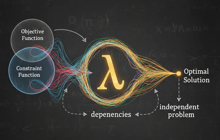
The Puzzle

When solving constrained optimization problems using Lagrange multipliers, something remarkable happens: we can take partial derivatives as if all variables are independent, even though the constraint actually makes them dependent on each other. How is this possible?

Let me walk you through the intuition and mathematics behind this elegant trick.

The Setup

Suppose we want to maximize $f(x,y)$ subject to a constraint $g(x,y) = 0$.

Normally, if you were to solve this directly, you might express $y$ as a function of $x$, writing $y = y(x)$, and then take:

$$\frac{d}{dx} f(x, y(x)) = \frac{\partial f}{\partial x} + \frac{\partial f}{\partial y} \frac{dy}{dx}$$

Here, the dependency of $y$ on $x$ matters explicitly, because the variables are not independent.

Enter the Lagrange Multiplier

Instead of dealing with this dependency directly, we define the Lagrangian:

$$\mathcal{L}(x, y, \lambda) = f(x, y) - \lambda g(x, y)$$

The key insight: we now treat $x$, $y$, and $\lambda$ as independent variables, even though $x$ and $y$ are actually linked by the constraint.

• $\lambda$ is the Lagrange multiplier
• It “absorbs” the effect of the constraint
• Taking partial derivatives with respect to $x$, $y$, and $\lambda$ ignores the dependency because the multiplier encodes it

The First-Order Conditions

We find critical points by setting all partial derivatives to zero:

$$\frac{\partial \mathcal{L}}{\partial x} = 0, \quad \frac{\partial \mathcal{L}}{\partial y} = 0, \quad \frac{\partial \mathcal{L}}{\partial \lambda} = 0$$

Let’s compute the first one explicitly:

$$\frac{\partial \mathcal{L}}{\partial x} = \frac{\partial}{\partial x}(f(x,y) - \lambda g(x,y))$$

By the rules of partial differentiation (treating $y$ and $\lambda$ as constants):

$$\frac{\partial \mathcal{L}}{\partial x} = \frac{\partial f}{\partial x} - \lambda \frac{\partial g}{\partial x}$$

Notice that:

• $\frac{\partial f}{\partial x}$ comes from differentiating $f(x,y)$ with respect to $x$
• $-\lambda \frac{\partial g}{\partial x}$ comes from differentiating $-\lambda g(x,y)$ with respect to $x$

Why This Works: The Two Approaches Compared

Let’s prove that the Lagrange multiplier method gives the same answer as computing the derivative along the constraint.

Approach 1: Along the Constraint

If we solve the constraint for $y = y(x)$ such that $g(x, y(x)) = 0$, the derivative of $f$ along the constraint is:

$$\frac{d}{dx} f(x, y(x)) = \frac{\partial f}{\partial x} + \frac{\partial f}{\partial y} \frac{dy}{dx}$$

To find $\frac{dy}{dx}$, we differentiate the constraint:

$$\frac{d}{dx} g(x, y(x)) = \frac{\partial g}{\partial x} + \frac{\partial g}{\partial y} \frac{dy}{dx} = 0$$

Solving for $\frac{dy}{dx}$:

$$\frac{dy}{dx} = -\frac{\partial g / \partial x}{\partial g / \partial y}$$

Substituting back:

$$\frac{d}{dx} f(x, y(x)) = \frac{\partial f}{\partial x} - \frac{\partial f}{\partial y} \frac{\partial g / \partial x}{\partial g / \partial y}$$

Approach 2: Lagrange Multiplier Method

From $\frac{\partial \mathcal{L}}{\partial y} = 0$:

$$\frac{\partial f}{\partial y} - \lambda \frac{\partial g}{\partial y} = 0 \implies \lambda = \frac{\partial f / \partial y}{\partial g / \partial y}$$

Substituting this into $\frac{\partial \mathcal{L}}{\partial x}$:

$$\frac{\partial \mathcal{L}}{\partial x} = \frac{\partial f}{\partial x} - \frac{\partial f / \partial y}{\partial g / \partial y} \frac{\partial g}{\partial x} = \frac{\partial f}{\partial x} - \frac{\partial f}{\partial y} \frac{\partial g / \partial x}{\partial g / \partial y}$$

The Match

These expressions are identical! The Lagrange multiplier approach automatically reproduces the derivative along the constraint, but without explicitly solving for the dependency.

The Intuition

Think of $\lambda$ as a “force” that enforces the constraint:

• Without the multiplier: You must solve $y(x)$ explicitly and plug it in
• With the multiplier: You pretend $x$ and $y$ are free, and $\lambda$ adjusts automatically to satisfy $g(x,y) = 0$

It’s like adding a virtual “tension” that keeps you on the constraint surface. The multiplier absorbs the dependency so you can work with simpler partial derivatives.

Key Takeaways

1. The Lagrange multiplier encodes the constraint’s effect on the optimization problem
2. We can treat variables as independent when computing partial derivatives of the Lagrangian
3. The method is equivalent to computing derivatives along the constraint, but more elegant
4. $\lambda$ has geometric meaning: It represents the rate of change of the optimal value with respect to relaxing the constraint

Conclusion

The beauty of Lagrange multipliers lies in this transformation: instead of dealing with messy dependencies explicitly, we introduce an auxiliary variable that absorbs these dependencies. This lets us work with simpler partial derivatives while still capturing the full structure of the constrained optimization problem.

Next time you set $\nabla \mathcal{L} = 0$, remember: you’re not ignoring the dependencies—the multiplier is handling them for you behind the scenes.

---

Want to explore more? Try working through a concrete example like maximizing $f(x,y) = xy$ subject to $x^2 + y^2 = 1$. You’ll see exactly how the multiplier absorbs the constraint!