🧬 Dynamic RNA velocity model-- (8) effective scVelo analysis

Introduction and GitHub repo

scVelo, like many other tools, like many other tools, computes mathematical models based on assumptions that are often unmet by real-world single-cell RNA-seq datasets.

Empowered by the in-depth conceptual and implementation foundations unveiled in my earlier blog posts, this post continues to explore effective applications of the dynamic RNA velocity model by:

Identifying key steps and parameters in scVelo pipeline and math models that are tunable to align with the mathematical foundations of dynamic RNA velocity model and to improve the estimation accuracy
Benchmarking strategies using simulated datasets with ground-truth velocities generated through state-of-the-art stochastic simulations
Revealing biologically significant tumor development trajectory by applying the strategies on real-world scRNAseq dataset
Providing tools to visualize the results and to generate heatmap that labels genes with known biological significance and highly correlated with latent time

The full code is available in my github repo

Run scVelo on simulated data

Wrangling the simulated data

Simulated data were downloaded here

I decide to:

store raw data in a layer
store spliced counts in both adata.X and adata.layers
store unspliced counts in adata.layers

It is according to the structure of scVelo object, said here

The current workflow works with the spliced counts in adata.X and expects the layers ‘unspliced’ and ‘spliced’. You can, of course, store the raw count matrix in adata.layers as well if you need it.

and scvelo stores unspliced and spliced counts (spliced both in adata.X and adata.layers)

b2b.layers['spliced'] = b2b.layers['counts_spliced']
b2b.layers['unspliced'] =b2b.layers['counts_unspliced']

Verify `milestone` and its relation to `traj_progression`

b2b.uns['traj_progressions']['edge'] = (
    b2b.uns['traj_progressions']['from'] + '->' + b2b.uns['traj_progressions']['to']
)

b2b.uns['traj_progressions']['edge'].index = [
    f"cell{int(i) + 1}" for i in b2b.uns['traj_progressions']['edge'].index
]

b2b.obs['edge']=b2b.uns['traj_progressions']['edge'].loc[b2b.obs['milestone'].index]

import pandas as pd
pd.crosstab(b2b.obs['milestone'], b2b.obs['edge']).T.to_csv(
    'milestone_edge_crosstab.csv', 
                       index=True,          
                       header=True,          
                       index_label='edge')

The result below shows the ground truth of the milestone trajectories, which contain two branches– A->B->D and A->C->E.

edge	A	B	C	D	E
left_sA->left_sB	219	0	0	0	0
left_sB->left_sBmid	53	0	0	0	0
left_sBmid->left_sC	0	151	0	0	0
left_sBmid->left_sD	0	0	146	0	0
left_sC->left_sEndC	0	0	0	201	0
left_sD->left_sEndD	0	0	0	0	223
right_sA->right_sB	231	0	0	0	0
right_sB->right_sBmid	52	0	0	0	0
right_sBmid->right_sC	0	140	0	0	0
right_sBmid->right_sD	0	0	149	0	0
right_sC->right_sEndC	0	0	0	194	0
right_sD->right_sEndD	0	0	0	0	241

Default scVelo pipeline fail to capture the ground truth

logging.info('1c.Preprocessing,PCA,findNeighbour,Calculate Moments')
scv.pp.filter_and_normalize(adata, min_shared_counts=20, n_top_genes=2000)
scv.pp.moments(adata, n_pcs=30, n_neighbors=30)

logging.info('1d.EM fitting and calculate scVelo dynamic RNA velocity')
scv.tl.recover_dynamics(adata,n_jobs=81)
scv.tl.velocity(adata, mode='dynamical')

logging.info('1e.calculate Markov chain of the differentiation process')
scv.tl.velocity_graph(adata)

logging.info("2.velocity embeding(independent of root cells)")
scv.pl.velocity_embedding_stream(adata, basis='umap',color='milestone',
                                 legend_loc='right margin',show=True,
                                 save='b2b_default_embedding.png')

logging.info('2a.infer root cell, and calculate gene-shared latent time corrected by neighborhood convolution')
scv.tl.latent_time(adata)# identical to recover_latent_time introduced in scVelo paper
scv.pl.scatter(adata, color='latent_time', color_map='gnuplot', size=80,dpi=300, show=True,
               save='b2b_default_latent-time.png')

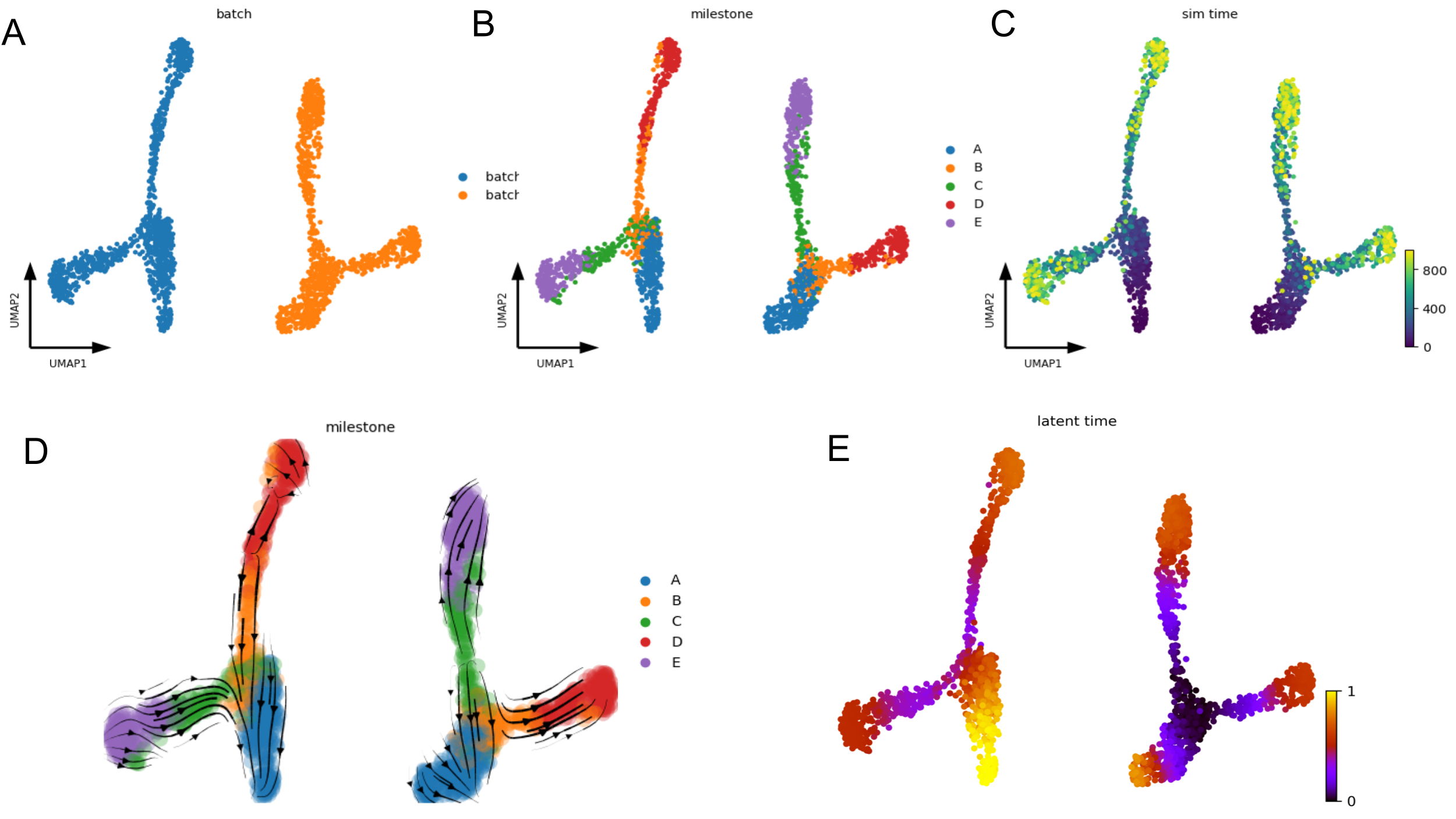
Below figures contain groud truth time of the cells in the SSA (Gillespie stochastic simulation algorithm) simulation (C) as well as the batch ID (A) and milestones (B). The velocity embedding stream (D) and latent time (E) plot clearly shows that the default scVelo pipeline fails to capture the ground truth of the bifurcation process, as the inferred velocity stream or latent time does not align with the known trajectories (A->B->D and A->C->E).

Default scVelo pipeline fail to capture the ground truth

scVelo performance depends on dataset ‘complexity’ and embedding space

Below are the velocity stream plots generated by scVelo when embedded in PCA space. ✔️ indicate successful recapitulation of the ground truth trajectories, while ❌ denote failure to recover the expected trajectories.

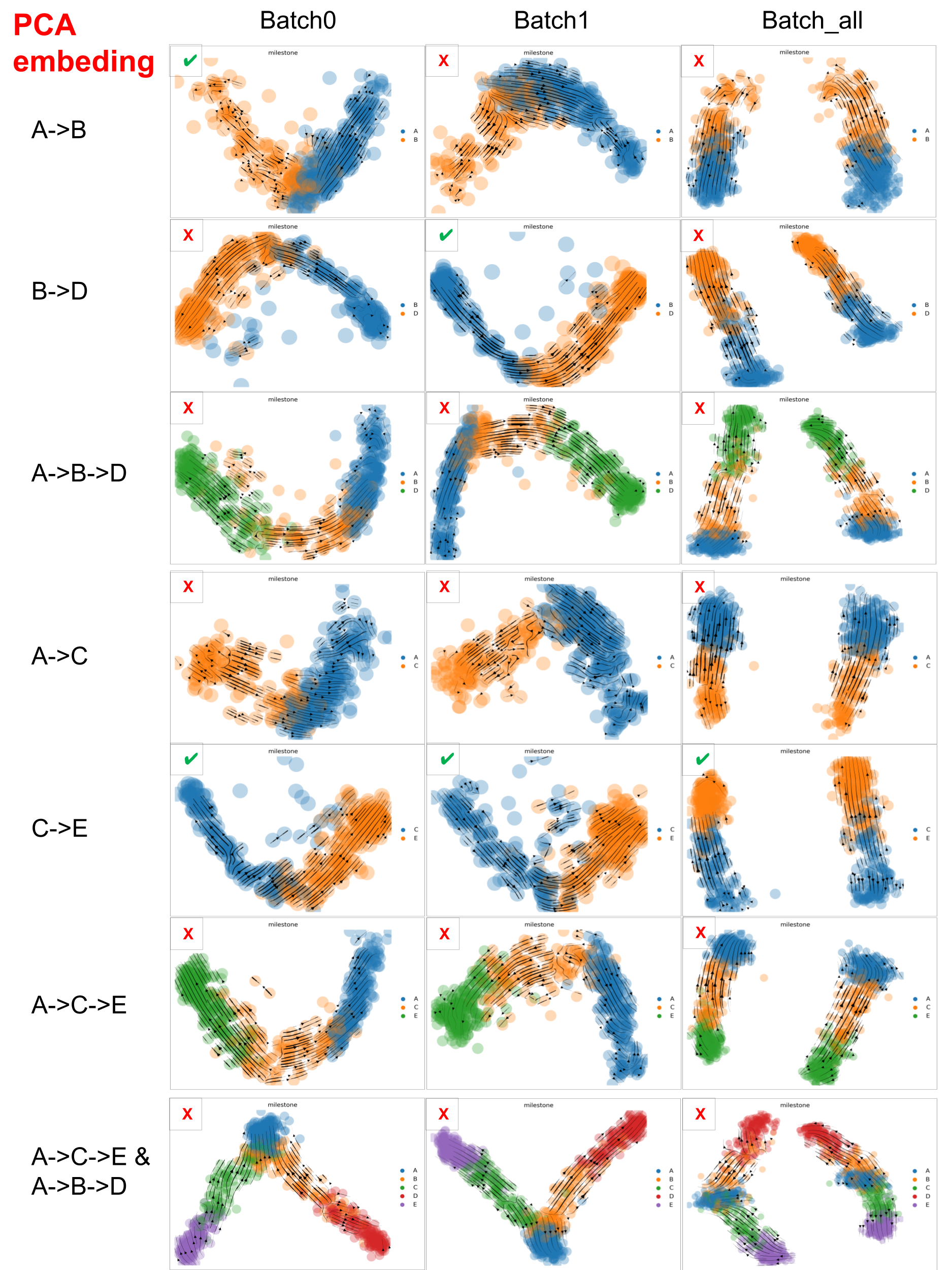
scVelo performance on datasets with varied ‘complexity’ in PCA space

Similarly, below are the Velocity stream plots from scVelo in UMAP space. ✔️ indicates successful trajectory recovery; ❌ denotes failure to match the ground truth.

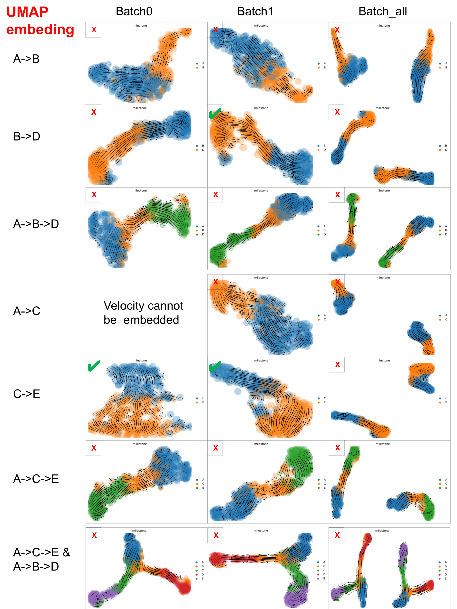
scVelo performance on datasets with varied ‘complexity’ in UMAP space

scVelo captured well the velocity of the dataset with minimal trajectory structures, such as A->B, B->D and C->E, but struggled with datasets that involve more complex trajectories.

And PCA embedding space is better than UMAP space, which may be due to the fact that PCA distorted data less than UMAP. But, especially for large scRNA-seq datasets, we have to consider that UMAP often resolves high-dimensional data better than PCA as PCA is linear, UMAP is nonlinear.

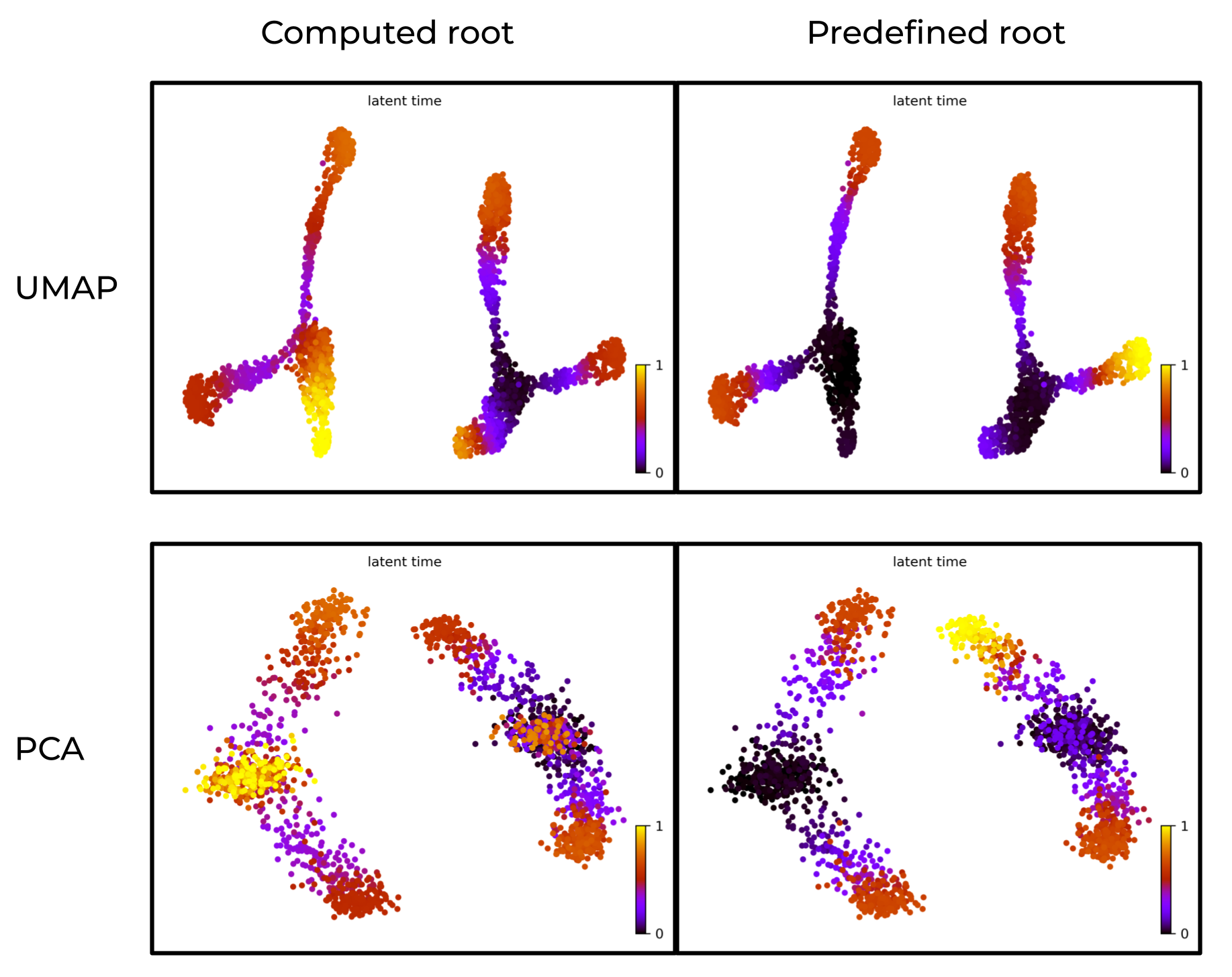
Prior knowledge of root cells improves accuracy of latent time

In below figure:

Left: scVelo-inferred latent time without prior knowledge of root cells.
Right: latent time with predefined root cells.

The right panel aligns better with the ground truth.

Prior knowledge of root cells improves accuracy of latent time

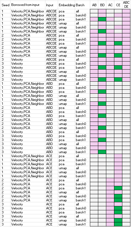
Borrow velocity, PCA and/or neighbor from larger population of cells

Below summarizes the performance of scVelo when borrowing velocity, PCA, and/or neighbor information from a larger population of cells. Speficically,

column ‘seed’ is the random seed used
column ‘borrowed from input’ is the items computed using the ‘input dataset’ and then used for the velocity analysis of the datasets specified by one of the names of the last five columns, i.e. one of ‘AB’, ‘BD’, ‘AC’, ‘CE’, or ‘ABCED’.
column ‘input’ is the ‘input dataset’
column ’emnbedding’ is the embedding space used for the velocity analysis, either PCA or UMAP
column ‘batch’ is the batch ID of the dataset
column ‘AB’, ‘BD’, ‘AC’, ‘CE’, or ‘ABCED’ are velocity analysis outcomes. Green indicates successful recovery of ground truth trajectories, pink denotes failure, and grey indicates the analysis could not be computed.

The results show that scVelo performs well when leveraging velocity, PCA and/or neighbor from larger populations, as ‘B->D’ and ‘C->E’ are able to recover the ground truth trajectories.

Later in this post, I will demonstrate that leveraging velocity, PCA, and/or neighborhood information from larger populations can effectively enhance the accuracy of velocity analysis in real-world, large-scale single-cell RNA-seq datasets.

Observations, mathematical and biological reasoning

1. unmet math assumptions underpinning scVelo’s failure to capture the ground truth by default

The default scVelo pipeline fails to capture the ground truth above. That is rooted into the unmet mathematical assumptions underpinning scVelo’s dynamic model, which include:

Constant gene-specific transcription rates (one for induction and one for repression), splicing, and degradation rates $\alpha$ ,$\beta$ ,$\gamma$ below are shared across cells. $$ \frac{du(t)}{dt} = \alpha^{(k)} - \beta u(t) $$ $$ \frac{ds(t)}{dt} = \beta u(t) - \gamma s(t) $$
Variance item in the likelihood to maximize is only dependent on gene and is shared across cells during parameter inference, consider $\sigma$ below is shared across cells. $$L(\theta) = \left(2\pi\sigma\right) \exp\left(-\frac{1}{2n\sigma^2}\sum_{i=1}^{n}(x_i^{\text{obs}} - x(t_i;\theta))^2\right)$$
Where:
- $L(\theta)$ is the likelihood function
- $\theta$ represents the parameters
- $\sigma$ is the standard deviation
- $n$ is the number of observations
- $x_i^{\text{obs}}$ are the observed values
- $x(t_i;\theta)$ are the model predictions at time $t_i$ given parameters $\theta$

These assumptions have not been validated for cells with different states, batches, or cell types as discussed by Gorin et. al., and strongly suggest calculating RNA velocity within a group of cells “similar” enough and avoiding mixing batch effects into the indeterminate biological noise. Dynamic model requires similarity of cells.

However, overly reducing the cell population to enforce similarity does not guarantee improved accuracy due to the potential bias introduced by small sample size. Please note. As a continuous and deterministic framework, the dynamic model is sensitive to the stochastic nature of scRNA-seq data.

In real-world applications, it is crucial to strike a balance: to find a scope that includes just enough cells so that the input cells are similar, yet still numerous enough to preserve reliable statistical properties (e.g., means, variances) required for the dynamic model to function effectively. And it is advisable to leverage velocity, PCA, and/or neighbor information from a larger population of cells to improve the accuracy of the dynamic model.

2. scVelo performance depends on dataset ‘complexity’ and embedding space

Consistent with the above discussion:

scVelo captured well the velocity of the dataset with minimal trajectory structures, such as A->B, B->D and C->E, but struggled with datasets that involve more complex trajectories.
The results show that scVelo performs better in PCA space than in UMAP space, which may be due to the fact that PCA distorted data less than UMAP. But we have to consider that UMAP often resolves high-dimensional data better than PCA as PCA is linear, UMAP is nonlinear.
- High-dimensional biological data (e.g., single-cell RNA-seq) often lies on nonlinear manifolds. UMAP can model this nonlinear structure, such as branching trajectories, subtle gradients, and clusters that PCA would flatten or blur.
scVelo performs well when borrowing velocity, PCA, and/or neighbor information from a larger population of cells, and later using real world scRNAseq data, we can see even improvement resulted from leveraging these calculations on a larger population of cells.

3. Prior knowledge of root cells is required

Without prior knowledge of root cells, there is no way to evaluate the accuracy of the inferred velocity stream to optimize the scope (the zoom-in extent) of the input cells.

Also, prior knowledge of root cells improve the accuracy of latent time computation.

Real-world data: tumor development

Integration or not?

We decide not to integrate different batches of data based on the mathematics defining the scVelo dynamic model and its inference as specifically disscussed above. No integration can perfectly seperate batch effects from biological noise yet.

Read mtx from star-velocyto into adata

adata_from_starsolo_mtx() import:

‘Gene/’+path_mtx + ‘matrix.mtx’ to adata.X
‘Velocyto/’+path_mtx+‘spliced.mtx’ to adata.layers[‘spliced’]
‘Velocyto/’+path_mtx+‘unspliced.mtx’ to adata.layers[‘unspliced’]
‘Velocyto/’+path_mtx+‘ambiguous.mtx’ to adata.layers[‘ambiguous’]

Key function is adata_from_starsolo_mtx() below, which reads the mtx files generated by STAR solo and stores them in an AnnData object. Please see other functions in the jupyter notebook in my github repo

import scvelo as scv
import scanpy as sc
import sys
import numpy as np
from scipy import sparse


def adata_from_starsolo_mtx(path_Solo_out='/data/wanglab_mgberis/UT_scRNAseq/starsolo_result/UT_ctrl/Solo.out/',
                            path_mtx='filtered/'):
    path=path_Solo_out
    ensure_file_format(path+'Gene/'+path_mtx)
    
    adata = sc.read_10x_mtx(path+'Gene/'+path_mtx)

    spliced=np.loadtxt(path+'Velocyto/'+path_mtx+'spliced.mtx', skiprows=3, delimiter=' ')
    shape = np.loadtxt(path+'Velocyto/'+path_mtx+'spliced.mtx', skiprows=2, max_rows = 1 ,delimiter=' ')[0:2].astype(int)

    adata.layers['spliced']=sparse.csr_matrix((spliced[:,2], (spliced[:,0]-1, spliced[:,1]-1)), shape = (shape)).tocsr().T

    unspliced=np.loadtxt(path+'Velocyto/'+path_mtx+'unspliced.mtx', skiprows=3, delimiter=' ')
    adata.layers['unspliced']=sparse.csr_matrix((unspliced[:,2], (unspliced[:,0]-1, unspliced[:,1]-1)), shape = (shape)).tocsr().T

    ambiguous= np.loadtxt(path+'Velocyto/'+path_mtx+'ambiguous.mtx', skiprows=3, delimiter=' ')
    adata.layers['ambiguous']=sparse.csr_matrix((ambiguous[:,2], (ambiguous[:,0]-1, ambiguous[:,1]-1)), shape = (shape)).tocsr().T
    
    return adata.copy()

Generate AnnData of all samples for scVelo

The Anndata object

stores spliced and unspliced counts from star using adata_from_starsolo_mtx() as discussed in Wrangling the simulated data
stores count data of seurat in layer X_fromSeurat
stores metadata of seurat

import os
import re
import scanpy as sc

for i, j in [
    ['CTR', 'UT_ctrl'],
    ['STU', 'UT_s'],
    ['BTU', 'UT_b']
]:
    print(f"h5ad label: {i}, starsolo label: {j}")
    
    output_file = f"{i}_for_scVelo.h5ad"
    if os.path.exists(output_file):
        print(f"{output_file} exists, skipping.")
        continue

    adata1 = sc.read_h5ad(f"{i}_RNA.h5ad")
    adata = adata_from_starsolo_mtx(f"/data/wanglab_mgberis/UT_scRNAseq/starsolo_result/{j}/Solo.out/")
    adata.layers["raw_counts"] = adata.X.copy()
    adata.X = adata.layers["spliced"].copy()

    for k in list(adata1.layers.keys()):
        print(f"shape of {k} is {adata1.layers[k].shape}")
    print(f"shape of X is {adata1.X.shape}")

    for k in list(adata.layers.keys()):
        print(f"shape of {k} is {adata.layers[k].shape}")
    print(f"shape of X is {adata.X.shape}")

    cell1 = [re.sub(r'_.*', '', x) for x in adata1.obs.index.tolist()]
    gene1 = adata1.var.index.tolist()
    cell_intersect = list(set(cell1) & set(adata.obs.index.tolist()))
    gene_intersect = list(set(gene1) & set(adata.var.index.tolist()))

    adata_sub = adata[cell_intersect, gene_intersect].copy()
    for k in list(adata_sub.layers.keys()):
        print(f"shape of {k} is {adata_sub.layers[k].shape}")
    print(f"shape of X is {adata_sub.X.shape}")

    adata1_sub = adata1[adata1.obs[adata1.obs['cell_name'].isin(cell_intersect)].index.tolist(),
                        gene_intersect].copy()
    for k in list(adata1_sub.layers.keys()):
        print(f"shape of {k} is {adata1_sub.layers[k].shape}")
    print(f"shape of X is {adata1_sub.X.shape}")

    for k in list(adata_sub.layers.keys()):
        adata1_sub.layers[k] = adata_sub.layers[k]
        print(f"adata1_sub layer {k} has been replaced by adata_sub.layers {k}")
    adata1_sub.layers['X_fromSeurat'] = adata1_sub.X
    adata1_sub.X = adata_sub.X
    print("adata1_sub X has been replaced by adata_sub X")

    # fix '_index' column name in raw.var if present
    adata1_sub.raw.var.rename(columns={'_index': 'index'}, inplace=True)
    adata1_sub.write(f"{i}_for_scVelo.h5ad")

Define experiment parameters

Key scripts are below and the full code is available in my github repo.

# =============================================================================
# CONFIGURATION PARAMETERS
# =============================================================================

# Task configuration: (h5ad filename prefix, whether to (re-)fit model, whether to save fitted output)
# Each tuple defines an analysis task with:
# - h5ad filename prefix: base name for input files (will look for {prefix}_for_scVelo.h5ad)
# - fit_bool: whether to rerun the full velocity fitting pipeline
# - save_bool: whether to save the fitted velocity model output
task_fit_save = [
    ['CTR',True,False],
    ['STU',True,False],
    ['BTU',True,False]
]

# Column name in adata.obs that contains cell group/type annotations
# Used for subsetting cells and defining root populations
root_config=['celltype.v2']
root_index_in_ss0=1
root_index_in_ss1=1

# Define cell population subsets for velocity analysis
# Each subset represents a group of cell types to analyze together
# Format: list of cell type identifiers that should exist in adata.obs[root_config[0]]
ss0_list = [
    ['tumor_1','tumor_Ki67+Ovgp1+'],
    ['tumor_1','tumor_Ki67+Ovgp1+','tumor_2'],
    ['tumor_1','tumor_Ki67+Ovgp1+','tumor_2','Epc','M','F'],
]

# The subset of elements of ss0_list. 
#  RNA velocity analysis on each subset will borrow info from its parant population
#  defined by the elements of ss0_list.
ss1_list = [
    [],
    [['tumor_1','tumor_Ki67+Ovgp1+']],
    [['tumor_1','tumor_Ki67+Ovgp1+']],
]

# Experimental configuration parameters for reproducibility and method comparison
# Each tuple contains: (random_seed, recompute_neighbors, recompute_PCA)
# - random_seed: ensures reproducible results across runs
# - recompute_neighbors: whether to recalculate neighborhood graph
# - recompute_PCA: whether to recalculate PCA embedding
seed_reNeibo_rePCA = [
    (1, False, False),
    # (2, True, False),
    # (3, True, True),
]

# Embedding methods to use for velocity projection
embed_basis=['pca','umap']

# Test the effect of redo dimension reduction for main set
re_dimRed_bool_list=[True,False]

# Define batches
adata.obs['batch'] =  adata.obs['orig.ident']
adata.obs['batch'] = adata.obs['batch'].astype('category')

# Set scVelo verbosity level (0=silent, 1=errors, 2=warnings, 3=info, 4=debug)
scv.settings.verbosity = 3

Key functions are below and the full code is available in my github repo.

def scvelo_classic_steps(subset, adata_name, seed, out_dir,
                         root_config=['milestone', ['A']],
                         embed_basis='umap'):
    """
    Execute the complete scVelo visualization and analysis pipeline.
    
    This function performs the main velocity analysis workflow:
    1. Generate basic embedding plots
    2. Compute velocity graph
    3. Create velocity vector field visualizations
    4. Infer latent time (pseudotime) with and without root cells
    5. Generate comprehensive result plots
    
    Parameters:
        subset : AnnData
            Preprocessed single-cell data subset
        adata_name : str
            Base name for output files
        seed : int
            Random seed for reproducibility
        out_dir : str
            Directory for saving results
        root_config : list, default=['milestone', ['A']]
            [column_name, [root_cell_types]] for latent time inference
        embed_basis : str, default='umap'
            Embedding method for visualization ('pca' or 'umap')
    """
    # Set output directories for scanpy and scvelo
    sc.settings.figdir = out_dir
    scv.settings.figdir = out_dir
    
    # Create descriptive filename components
    celltypes = "".join(sorted(subset.obs[root_config[0]].unique().tolist()))
    i = adata_name
    
    # Select appropriate plotting function
    pl_func = {
        "umap": sc.pl.umap,
        "pca": sc.pl.pca
    }
    
    # =========================================================================
    # 1. BASIC EMBEDDING VISUALIZATION
    # =========================================================================
    log_n_print(f"1a. Generating {embed_basis} embedding plot")
    pl_func[embed_basis](
        subset,
        color=root_config[0],
        frameon=False,
        legend_loc='right margin',
        show=False,
        title=i,
        save=f"{i}_{celltypes}_{embed_basis}_seed{seed}.png",
    )

    # =========================================================================
    # 2. VELOCITY GRAPH COMPUTATION
    # =========================================================================
    velocity_error = None
    try:
        scv.tl.velocity_graph(subset)
        log_n_print("Velocity graph computed successfully")
    except Exception as e:
        velocity_error = e
        log_n_print("Error computing velocity graph:")
        log_n_print(str(e))
    
    # =========================================================================
    # 3. VELOCITY VISUALIZATIONS (only if graph computation succeeded)
    # =========================================================================
    if velocity_error is None:
        log_n_print('3a. Generating velocity embedding plot')
        
        # Clear any existing velocity embedding
        subset.obsm.pop('velocity_umap', None)
        
        # Compute velocity embedding
        scv.tl.velocity_embedding(subset, basis=embed_basis)
        
        # Plot velocity vectors on embedding
        scv.pl.velocity_embedding(
            subset,
            basis=embed_basis,
            color=root_config[0],
            arrow_length=1,
            arrow_size=3,
            dpi=300,
            frameon=False,
            show=False,
            save=f"{i}_{celltypes}_velocity_embedding_seed{seed}.pdf",
        )
        
        # =====================================================================
        # 3b. VELOCITY STREAM PLOT
        # =====================================================================
        log_n_print('3b. Generating velocity stream plot')
        try:
            scv.pl.velocity_embedding_stream(
                subset,
                basis=embed_basis,
                dpi=300,
                color=root_config[0],
                show=False,
                legend_loc='right margin',
                save=f"{i}_{celltypes}_velocity_embedding_stream_seed{seed}.png",
            )
        except Exception as e1:
            log_n_print("Error in velocity_embedding_stream (first attempt):")
            log_n_print(str(e1))
            
            # Try with recomputation
            try:
                log_n_print("Attempting stream plot with recomputation...")
                scv.pl.velocity_embedding_stream(
                    subset,
                    basis=embed_basis,
                    dpi=300,
                    recompute=True,
                    color=root_config[0],
                    show=False,
                    legend_loc='right margin',
                    save=f"{i}_{celltypes}_velocity_embedding_stream_recomputed_seed{seed}.png",
                )
            except Exception as e2:
                log_n_print("Error in velocity_embedding_stream (even after recomputation):")
                log_n_print(str(e2))
                log_n_print("Skipping stream plot for this subset")
        
        # =====================================================================
        # 4. LATENT TIME INFERENCE
        # =====================================================================
        
        # 4a. Latent time without root cell specification
        log_n_print('4a. Inferring latent time without root cell specification')
        
        # Clean any existing root cell annotations
        if 'root_cells' in subset.obs:
            del subset.obs['root_cells']
        
        # Compute latent time (pseudotime) based on velocity
        scv.tl.latent_time(subset)
        
        # Plot latent time without root
        scv.pl.scatter(
            subset,
            basis=embed_basis,
            color='latent_time',
            show=False,
            color_map='gnuplot',
            size=80,
            dpi=300,
            save=f"{i}_{celltypes}_latent_time_noRoot_seed{seed}.png",
        )
        
        # 4b. Latent time with root cell specification
        log_n_print('4b. Defining root cells and recomputing latent time')
        
        # Define root cells based on cell type annotation
        # Uses the first cell type in sorted order as root
        root_cells = subset.obs_names[subset.obs[root_config[0]].isin(root_config[1])]
        subset.obs['root_cells'] = subset.obs_names.isin(root_cells)
        
        log_n_print(f'Root cells defined as: {root_config[1]} ({len(root_cells)} cells)')
        
        # Recompute latent time with root cell constraint
        scv.tl.latent_time(subset, root_key='root_cells')
        
        # Plot latent time with root specification
        scv.pl.scatter(
            subset,
            basis=embed_basis,
            color='latent_time',
            color_map='gnuplot',
            size=80,
            dpi=300,
            show=False,
            save=f"{i}_{celltypes}_latent_time_AAsRoot_seed{seed}.png",
        )
        
        log_n_print(f'Completed velocity analysis for {celltypes}')

Iterate through experimental configurations

Below is excerpt of the code that run the scVelo analysis pipeline for each combination of tasks and experimental configurations. The full code is available in my github repo.

# =============================================================================
# Configure logging
#  loging all parameters and tasks to help debugging and reproducibility
# =============================================================================

# refer to my github repo for the full code

# =============================================================================
# Iterate through all combinations of tasks and experimental configurations
# same as for simulated data except here also test the effect of redo dimension reduction for main set
# =============================================================================

for (i, fit_bool, save_bool), (seed, reNeibor_bool, rePCA_bool) in product(task_fit_save, seed_reNeibo_rePCA):
    
    # Set random seeds for reproducibility
    random.seed(seed)
    np.random.seed(seed)
    
    # Log current processing parameters
    log_n_print(f"---")
    log_n_print(f"Task(h5ad label): {i}, Fit: {fit_bool}, Save: {save_bool}")
    log_n_print(f"Seed: {seed}, reNeibor_bool: {reNeibor_bool}, rePCA_bool: {rePCA_bool}")
    
    # Clean up previous adata object to save memory
    if 'adata' in locals():
        del adata
    
    # 1. Load input data
    log_n_print('1.input')
    adata = sc.read_h5ad(f"{i}_for_scVelo.h5ad")  # Load pre-processed velocity data
    adata = clean_velocity_legacy(adata)           # Clean legacy velocity annotations
    
    # 2. Handle batch processing
    # Process each batch separately plus all batches combined
    if 'batch' in adata.obs:
        batch_list = list(adata.obs['batch'].cat.categories) + ['all']
    else:
        batch_list = ['all']
    
    # Process each batch
    for batch_ in batch_list:
        if batch_ == 'all':
            adata_batch = adata
            batch_1 = 'all'
        else:
            adata_batch = adata[adata.obs['batch'] == batch_]
            batch_1 = batch_.replace(' ', '')  # Remove spaces for file naming
        
        # 3. Process cell type subsets
        for ss0, ss1 in zip(ss0_list, ss1_list):
            
            # Filter for specified cell types in ss0
            adata1 = adata_batch[adata_batch.obs[root_config[0]].isin(ss0)]
            
            # Test with and without redoing dimensionality reduction
            for re_dimRed_bool in re_dimRed_bool_list:
                adata2 = adata1.copy()
                
                # Optionally redo dimensionality reduction
                if re_dimRed_bool:
                    log_n_print(f"<---redo dimension reduction--->")
                    sc.tl.pca(adata2)        # Principal component analysis
                    sc.pp.neighbors(adata2)   # Compute neighborhood graph
                    sc.tl.umap(adata2)       # UMAP embedding
                
                # Apply scVelo preprocessing
                adata2 = scvelo_pp(adata2, save_bool, ss0)
                
                # 4. Process different embedding bases (PCA and UMAP)
                for embed_basis_ in embed_basis:
                    
                    # Generate output directory name
                    out_dir_ = eval_out_dir(i, ss0, seed, embed_basis_, batch_1, reNeibor_bool, rePCA_bool)
                    
                    # Run main scVelo analysis pipeline
                    scvelo_classic_steps(
                        subset=adata2,
                        embed_basis=embed_basis_,
                        adata_name=i,
                        seed=seed,
                        out_dir=out_dir_,
                        root_config=[root_config[0], [sorted(ss0)[root_index_in_ss0]]],
                        re_dimRed_bool=re_dimRed_bool
                    )
                    
                    # 5. Process secondary subsets (ss1) if they exist
                    # This allows borrowing information from parent population
                    # while focusing analysis on specific sub-populations
                    for ss1_ in ss1:
                        # Filter for ss1 cell types and clear velocity graph
                        adata3 = clear_velocity_graph(adata2[adata2.obs[root_config[0]].isin(ss1_)])
                        
                        # Run scVelo analysis on subset with optional reprocessing
                        scvelo_classic_steps(
                            subset=reNeibor_rePCA(adata2=adata3, reNeibor_bool=reNeibor_bool, rePCA_bool=rePCA_bool),
                            embed_basis=embed_basis_,
                            adata_name=i,
                            seed=seed,
                            out_dir=out_dir_,
                            root_config=[root_config[0], [sorted(ss1_)[root_index_in_ss1]]],
                            re_dimRed_bool=re_dimRed_bool
                        )

Interim results

Below shows that leveraging velocity, PCA and/or neighbor from tumor population of cells enables scVelo to recapiculate a biologically meaningful tumor development trajectory, tumor_Ki67+Ovgp1+ -> tumor_1.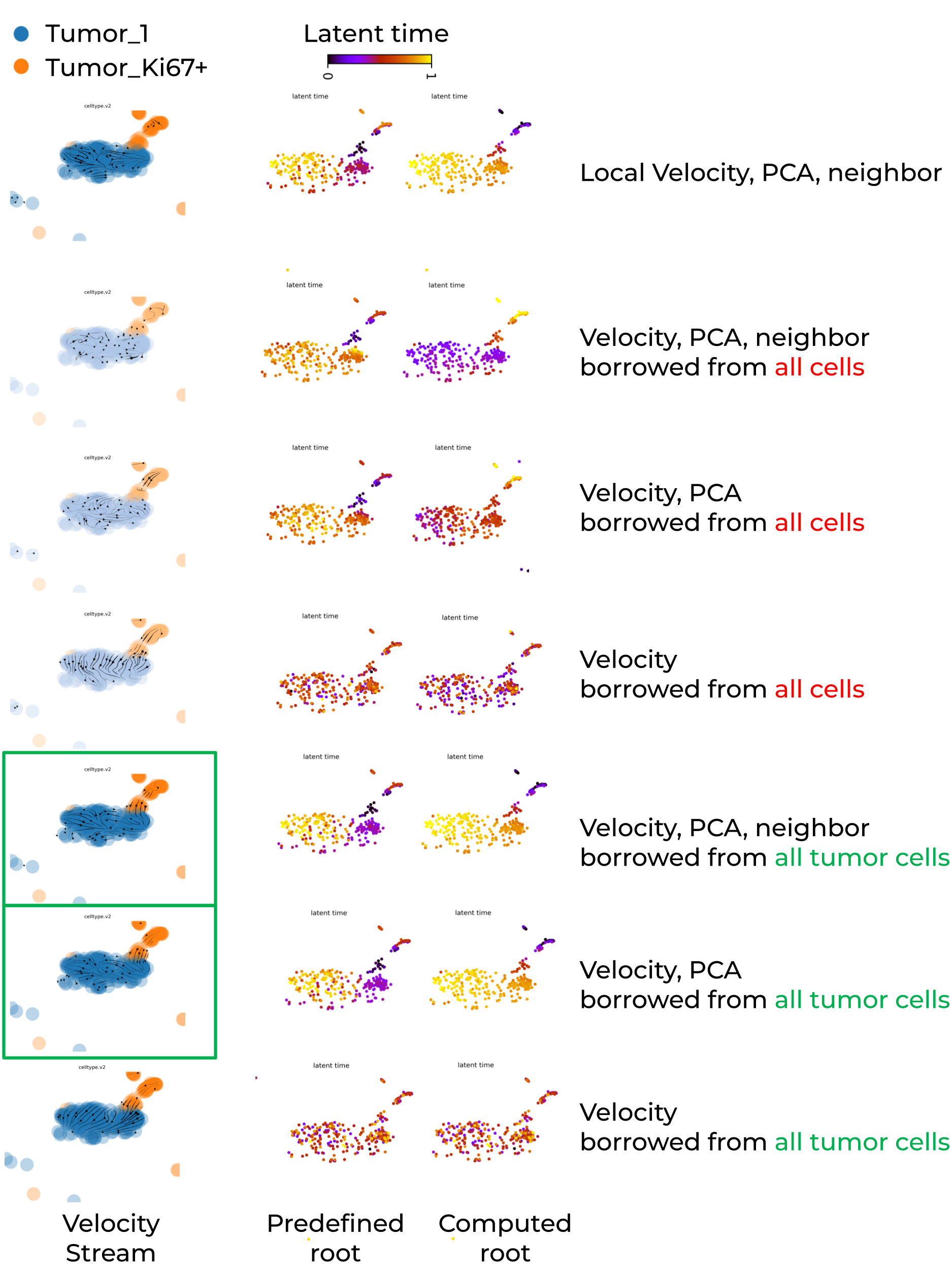

Key summary are:

Global PCA embedding space mixed cells from different trajectory locations, whereas global UMAP embedding space successfully separated them.
Locally recomputed UMAP failed to maintain trajectory separation, instead mixing cells from different trajectory regions.
If embedding space separated cells far away, dynamic model or any continuous model struggle to capture meaningful transition (e.g., velocity stream inference).
Whenver its possible, run scVelo on individual batch to avoid batch-induced artifacts.
Reduce the number of cell types in the input dataset to enforce greater cell-state similarity, and leverage velocity, PCA, or neighbor information from a larger reference population to improve the statistical robustness of velocity estimation in large-scale single-cell RNA-seq datasets.
Prior knowledge of root cells is required to evaluate the accuracy of the inferred velocity stream and to improve the accuracy of latent time computation.

Heatmap of biologically significant genes assocated with latent time

The default scVelo heatmap is pretty but it dose not label genes, and the color bar is not restored. Below are customized scripts to generate heatmap that labels the genes with known biological significance and highly correlated with latent time. The customized heatmap alsp restores the color bar and group legend.

Rank genes by correlation with latent time

Key function L_rank_genes_by_latent_time() and other ccodes is available in my github repo.

Customized heatmap to label selected genes and restore color bar, group legend

def L_scv_pl_heatmap(
    adata,
    var_names,
    sortby="latent_time",
    layer="Ms",
    color_map="viridis",
    col_color=None,
    palette="viridis",
    n_convolve=30,
    standard_scale=0,
    sort=True,
    colorbar=None,
    col_cluster=False,
    row_cluster=False,
    context=None,
    font_scale=None,
    figsize=(8, 4),
    show=None,
    save=None,
    debug=False,
    label_genes=None,
    min_label_spacing = 0.1,
    x_outside = 1.1,
    print_actual_gene_order = False,
    **kwargs,
):
    """
    Plot a heatmap of gene expression across latent time using seaborn's clustermap,
    with optional smoothing, sorting, column color annotations, and external gene labels.

    Parameters
    ----------
    adata : AnnData
        Annotated data matrix from scVelo or Scanpy with expression and metadata.
    
    var_names : list of str
        List of gene names to include in the heatmap (must exist in `adata.var_names`).
    
    sortby : str, default "latent_time"
        Observation key to use for sorting cells (e.g., pseudotime).
    
    layer : str, default "Ms"
        Layer of `adata` to use for expression values (e.g., spliced, unspliced, total).
    
    color_map : str, default "viridis"
        Colormap to use for the heatmap.
    
    col_color : str or list of str, optional
        Keys from `adata.obs` to add as categorical top bars in the heatmap.
    
    palette : str, default "viridis"
        Color palette to use for categorical color annotations.
    
    n_convolve : int or None, default 30
        If set, smooth expression along pseudotime using a moving average of this window size.
    
    standard_scale : int (0 or 1), default 0
        Whether to standardize across rows (0) or columns (1).
    
    sort : bool, default True
        Whether to sort genes by the peak time of expression.
    
    colorbar : bool or None
        Whether to display the expression colorbar.
    
    col_cluster : bool, default False
        Whether to cluster columns (cells).
    
    row_cluster : bool, default False
        Whether to cluster rows (genes).
    
    context : str or None
        Seaborn context (e.g., "notebook", "talk", "poster") for font scaling.
    
    font_scale : float or None
        Font scaling factor for seaborn context.
    
    figsize : tuple, default (8, 4)
        Size of the figure in inches.
    
    show : bool or None
        Whether to show the plot immediately.
    
    save : str or None
        Path to save the plot if desired.
    
    debug : bool, default False
        If True, prints intermediate data for debugging.
    
    label_genes : list of str or None
        Subset of genes to label outside the heatmap with connecting lines.
    
    min_label_spacing : float, default 0.1
        Minimum vertical spacing between gene labels (in Axes coordinates).
    
    x_outside : float, default 1.1
        Horizontal position to place gene labels outside the heatmap (Axes coordinates).
    
    print_actual_gene_order : bool, default False
        If True, prints the actual gene order used in the heatmap after clustering.

    Returns
    -------
    cm : seaborn.matrix.ClusterGrid or None
        The ClusterGrid object representing the heatmap (only returned if show=False).
    """
        
    import seaborn as sns
    import numpy as np
    import pandas as pd
    from scipy.sparse import issparse

    from scvelo import logging as logg
    from scvelo.tools.utils import strings_to_categoricals
    from scvelo.utils import (
        interpret_colorkey,
        is_categorical,
    )
    from scvelo.plotting.utils import (
        savefig_or_show,
        set_colors_for_categorical_obs,
        to_list,
    )

    var_names = [name for name in var_names if name in adata.var_names]
    if not var_names:
        logg.error("No valid genes found in `adata.var_names` for plotting. Please check your `var_names` input.")
        return # Or raise an error

    tkey, xkey = kwargs.pop("tkey", sortby), kwargs.pop("xkey", layer)
    time = adata.obs[tkey].values
    valid = np.isfinite(time)
    if not np.any(valid):
        logg.error(f"No finite values found in adata.obs['{tkey}']. Cannot sort and plot.")
        return
    time = time[valid]

    X = (
        adata[:, var_names].layers[xkey]
        if xkey in adata.layers.keys()
        else adata[:, var_names].X
    )
    if issparse(X):
        X = X.toarray()
    X = X[valid]
    if debug:
        print("X is:")
        print(X)
    df = pd.DataFrame(X[np.argsort(time)], columns=var_names)
    if debug:
        print('before setting index')
        print(df)
    df.index = adata.obs_names[valid][np.argsort(time)]
    if debug:
        print('after setting index')
        print(df)

    if n_convolve is not None:
        weights = np.ones(n_convolve) / n_convolve
        for gene in var_names:
            try:
                df[gene] = np.convolve(df[gene].values, weights, mode="same")
            except ValueError as e:
                logg.info(f"Skipping variable {gene}: {e}")
                pass

    if sort:
        max_sort = np.argsort(np.argmax(df.values, axis=0))
        if debug:
            print('if sort w/o index')
            print(pd.DataFrame(df.values[:, max_sort], columns=df.columns[max_sort]))
        df = pd.DataFrame(df.values[:, max_sort], columns=df.columns[max_sort], index=df.index)
        if debug:
            print('sorted w index')
            print(df)

    strings_to_categoricals(adata)

    #<===== Handle multiple col_color keys as a DataFrame of color tracks =====>
    if col_color is not None:
        original_col_color_keys = to_list(col_color)
        col_color_dict = {}
    else:
        original_col_color_keys = None

    if original_col_color_keys is not None:
        for col in original_col_color_keys:
            if not is_categorical(adata, col):
                obs_col = adata.obs[col]
                cat_col = np.round(obs_col / np.max(obs_col), 2) * np.max(obs_col)
                adata.obs[f"{col}_categorical"] = pd.Categorical(cat_col)
                col += "_categorical"
                set_colors_for_categorical_obs(adata, col, palette)
            col_color_dict[col] = interpret_colorkey(adata, col)[np.argsort(time)]
        col_colors = pd.DataFrame(col_color_dict, index=adata.obs_names[valid][np.argsort(time)])# Combine all into a DataFrame for seaborn
    
    #<=== below set cbar_pos required for colorbar ===>
    if "cbar_pos" not in kwargs:
        kwargs["cbar_pos"] = (0.02, 0.8, 0.03, 0.18) if colorbar is not False else None
    kwargs.setdefault("cbar_kws", {"label": "expression"})

    args = {}
    if font_scale is not None:
        args = {"font_scale": font_scale}
        context = context or "notebook"

    with sns.plotting_context(context=context, **args):
        if debug:
            print(f"Shape of col_colors DataFrame: {col_colors.shape}")
            print(f"Number of NaN values in col_colors: {col_colors.isnull().sum().sum()}")
            print(f"Are col_colors empty? {col_colors.empty}")
            print(f"col_colors: {col_colors}")
            print(f"DataFrame shape before clustermap: {df.shape}")
            print(f"Number of NaN values in df: {df.isnull().sum().sum()}")
        
        #<=== below enable col_colors is rendered as the top bar ===>
        col_colors = col_colors.loc[df.index]
        
        #<=== remove the label of catagory bar "col_colors" ===>
        col_colors.columns = [""]
        
        kwargs.update(
            {
                "col_colors": col_colors,
                "col_cluster": col_cluster,
                "row_cluster": row_cluster,
                "cmap": color_map,
                "xticklabels": False,
                "standard_scale": standard_scale,
                "figsize": figsize,
            }
        )

        try:
            cm = sns.clustermap(df.T, **kwargs)
        except ImportWarning:
            logg.warn("Please upgrade seaborn with `pip install -U seaborn`.")
            kwargs.pop("dendrogram_ratio")
            kwargs.pop("cbar_pos")
            cm = sns.clustermap(df.T, **kwargs)
        
        #<=== remove top tick marks of catagory bar "col_colors" ===>
        if hasattr(cm, "ax_col_colors"):
            cm.ax_col_colors.set_yticks([])
        
        #<=== Specify the genes to label ===>
        L_add_gene_labels(cm, df, label_genes,
                           min_label_spacing = min_label_spacing,
                           x_outside = x_outside,
                           print_actual_gene_order = print_actual_gene_order
                          )
       
        #<=== Manually add legends for categorical col_colors ===>
        if original_col_color_keys is not None:
            import matplotlib.patches as mpatches
            for col, color_array in zip(original_col_color_keys, col_colors):
                if is_categorical(adata, col):
                    categories = adata.obs[col].cat.categories
                    colors = adata.uns.get(f"{col}_colors", [])
                    if categories is not None and colors is not None:
                        handles = [
                            mpatches.Patch(color=c, label=cat)
                            for cat, c in zip(categories, colors)
                        ]
                        cm.ax_col_dendrogram.legend(
                            handles=handles,
                            title=col,
                            bbox_to_anchor=(1.05, 1),
                            loc="upper left",
                            fontsize="small",
                            frameon=False,
                        )

    savefig_or_show("heatmap", save=save, show=show, dpi=300)
    if show is False:
        return cm


def L_add_gene_labels(cm, df, label_genes,
                        min_label_spacing,
                        x_outside,
                        print_actual_gene_order
                          ):
    """
    Add gene labels outside the heatmap along the Y-axis with repelling to reduce overlap.

    This function uses Axes coordinates to place gene names outside the heatmap and
    draws connecting lines to the actual rows. It avoids overlap by pushing labels apart
    vertically while preserving order.

    Parameters
    ----------
    cm : seaborn.matrix.ClusterGrid
        The heatmap object generated by seaborn.clustermap.

    df : pd.DataFrame
        The gene expression data used in the heatmap, with genes in columns.

    label_genes : list of str
        Genes to label outside the heatmap. Only those in `df.columns` are considered.

    min_label_spacing : float
        Minimum spacing between labels (in Axes coordinate units). Helps avoid overlap.

    x_outside : float
        Horizontal position to place labels (Axes coordinate system, >1 means right of heatmap).

    print_actual_gene_order : bool
        If True, prints the actual row order of genes after any reordering done by clustering.

    Returns
    -------
    None
        This function modifies the heatmap in-place by adding text and annotation lines.
    """
    if label_genes is None:
        return
        
    label_set = set(label_genes)
    
    # Get the actual row order from the clustermap object
    # This accounts for any reordering done by seaborn during plotting
    if hasattr(cm, 'dendrogram_row') and cm.dendrogram_row is not None:
        # If row clustering was used, get the reordered indices
        row_order = cm.dendrogram_row.reordered_ind
        actual_gene_order = [df.columns[i] for i in row_order]
    else:
        # No row clustering, use the original order
        actual_gene_order = df.columns.to_list()
    
    if print_actual_gene_order:
        print(actual_gene_order)
    # Find positions of labeled genes in the ACTUAL display order
    labeled_genes_data = []
    for i, gene in enumerate(actual_gene_order):
        if gene in label_set:
            gene_y_coord = 1.0 - (i + 0.5) / len(actual_gene_order)
            labeled_genes_data.append({
                'gene': gene,
                'gene_row_index': i,
                'gene_y_coord': gene_y_coord,  # Where the gene actually is
                'label_y_coord': gene_y_coord  # Where we'll put the label (initially same)
            })
    
    # Apply repulsion to avoid overlapping labels
    if len(labeled_genes_data) > 1:
        total_height = len(actual_gene_order)
        
        # Sort by gene position
        labeled_genes_data.sort(key=lambda x: x['gene_y_coord'], reverse=True)
        
        # Adjust label positions to avoid overlap while keeping them in order
        for i in range(1, len(labeled_genes_data)):
            prev_label_y = labeled_genes_data[i-1]['label_y_coord']
            curr_label_y = labeled_genes_data[i]['label_y_coord']
            
            # If labels would overlap, move the current one down
            if prev_label_y - curr_label_y < min_label_spacing:
                labeled_genes_data[i]['label_y_coord'] = prev_label_y - min_label_spacing
        
        # Make sure no labels go below 0
        for i in range(len(labeled_genes_data)):
            if labeled_genes_data[i]['label_y_coord'] < 0:
                labeled_genes_data[i]['label_y_coord'] = 0
    
    # Add the labels and connecting lines

    for gene_data in labeled_genes_data:
        gene = gene_data['gene']
        gene_y = gene_data['gene_y_coord']  # Where the gene row actually is
        label_y = gene_data['label_y_coord']  # Where we'll place the label
        
        # Add the text label (potentially moved to avoid overlap)
        cm.ax_heatmap.text(
            x_outside,
            label_y,
            gene,
            fontsize=8,
            ha="left",
            va="center",
            transform=cm.ax_heatmap.transAxes,
            bbox=dict(facecolor='none', edgecolor='black', alpha=0.5, pad=1),
            clip_on=False
        )
        
        # Add a line connecting the label to the ACTUAL gene row
        cm.ax_heatmap.annotate(
            '',
            xy=(1.0, gene_y),  # Points to the actual gene row
            xytext=(x_outside - 0.002, label_y),  # Comes from the label position
            xycoords='axes fraction',
            textcoords='axes fraction',
            arrowprops=dict(arrowstyle='-', color='black', lw=0.5),
            clip_on=False
        )

Heatmap highlighting latent-time correlated genes with known biological significance

Below shows the root cells (tumor_Ki67+Ovgp1+) expressed highly genes associated with stemness and proliferation, such as Mki67, Ezh2, B2m and Pdgfra, while tumor_1 cells have more terminal differentiated gene expression.

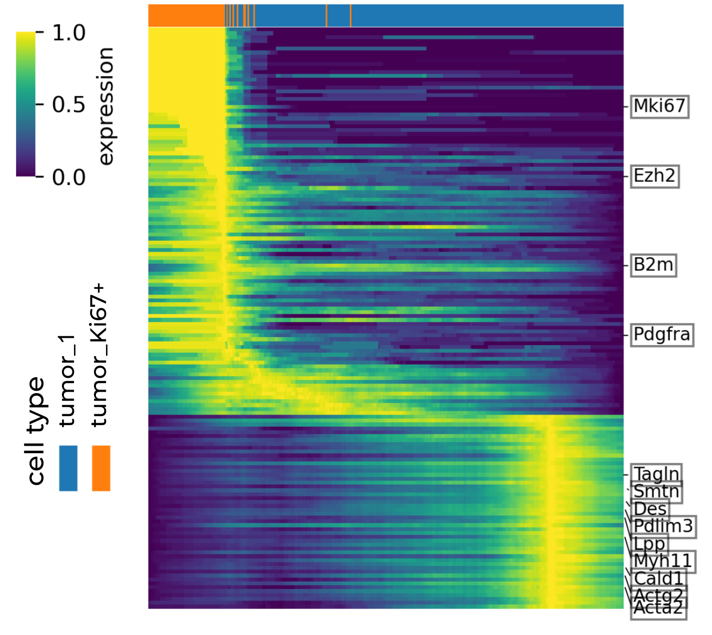
Heatmap of genes associated with latent time