💨 Modeling the deposition of infectious agents suggests that aerosolized drugs offer enhanced specificity
 Image credit: Andrey Soldatov on Unsplash
Github source code
please see source codes in github.
Introduction
Alveolar deposition is indeed a key event in respiratory infections, including pneumonia and viral infections like COVID-19. It allows many infectious agents (like bacteria, viruses, and fungi) to establish infection and cause damage to the lungs and overall health. Aerosols of 1–5 microns in diameter are able to bypass the upper airways and reach the deep parts of the lungs, including the alveoli. It is through aerosols that respiratory diseases like COVID-19, tuberculosis, and influenza spread so effectively.
I thought the small size of aerosols that deeply reach alveoli made them subject to Brownian motion and deposit in a random, erratic pattern. But the Fig 1D of Rothchild et al.,(2019) strongly challenged this idea. Specifically, the mice were infected with 2 × 10³ aerosolized tuberculosis bateria (M.tb), and one day later more than 15% of the infected alveoli contained two bacteria. Considering the 36-hour douling time of M.tb even in rich growth conditions, we can reasonably ignore M.tb proliferation within the first day, during which the bacteria must acclimate to the immunocompetent lung environment. The frequency, therefore, does not align with the assumption that M.tb deposits randomly in each infection niche—the region surveilled by one of the more than 7 × 10⁵ individual alveolar macrophages—at the same probability.
I will demonstrate below that random niche deposition cannot recapitulate the results shown in Fig 1D, however, preferential deposition in certain niches successfully reproduces the findings. This suggests that infectious agents affect alveoli unevenly, and precision medicine should account for this variability to achieve satisfactory specificity and efficacy. Aerosolized drugs with similar deposition patterns are expected to be more advantageous compared to the same drugs delivered by other routes. Also please see source codes in github.
Random deposition
Assume each droplet deposit in alveolar niches independently and all niches ($N_{niche}$ is total number of niches) have the same probability $p$ to receive the M.tb. Thus $$ p N_{niche} = 1 $$ Below R codes applied Monte Carlo simulation one million times for each scenario, traversing the parameter space where the niche population size is $N_{niche} \in [0.1, 2.4] \times 10^6$ , and the total number of M. tuberculosis (M.tb) deposited in the alveoli is $n_{Mtb} \in [2, 4] \times 10^3$ .
#faster Monte_Carlo
Monte_Carlo_1<- function (CFU, nAlveoli, nSim=1e6,extraLabel=""){
	  t1<-integer(3);
	  names(t1)<-c("nNicheOccupiedBy1Bug","nNicheOccupiedBy2Bug",
	  "nNicheOccupiedByMore")
  for (i in 1:nSim) {
  	t<-table(sample(1L: nAlveoli, CFU, replace=T))
  	t1[1]<-t1[1]+as.integer(sum(t==1L))
  	t1[2]<-t1[2]+as.integer(sum(t==2L))
  	t1[3]<-t1[3]+as.integer(sum(t>2L))
  	}
  saveRDS(t,paste0("CFU", CFU, ",nAlveoli", nAlveoli,".rds"))
}
for (CFU in seq.int(2e3,4e3,1e2)) {
  for (nAlveoli in seq.int(1e5,2.4e6,1e5)){
    tm<-proc.time()
    Monte_Carlo_1(CFU,nAlveoli,extraLabel="_1",)
    proc.time()-tm
  }
}
Result
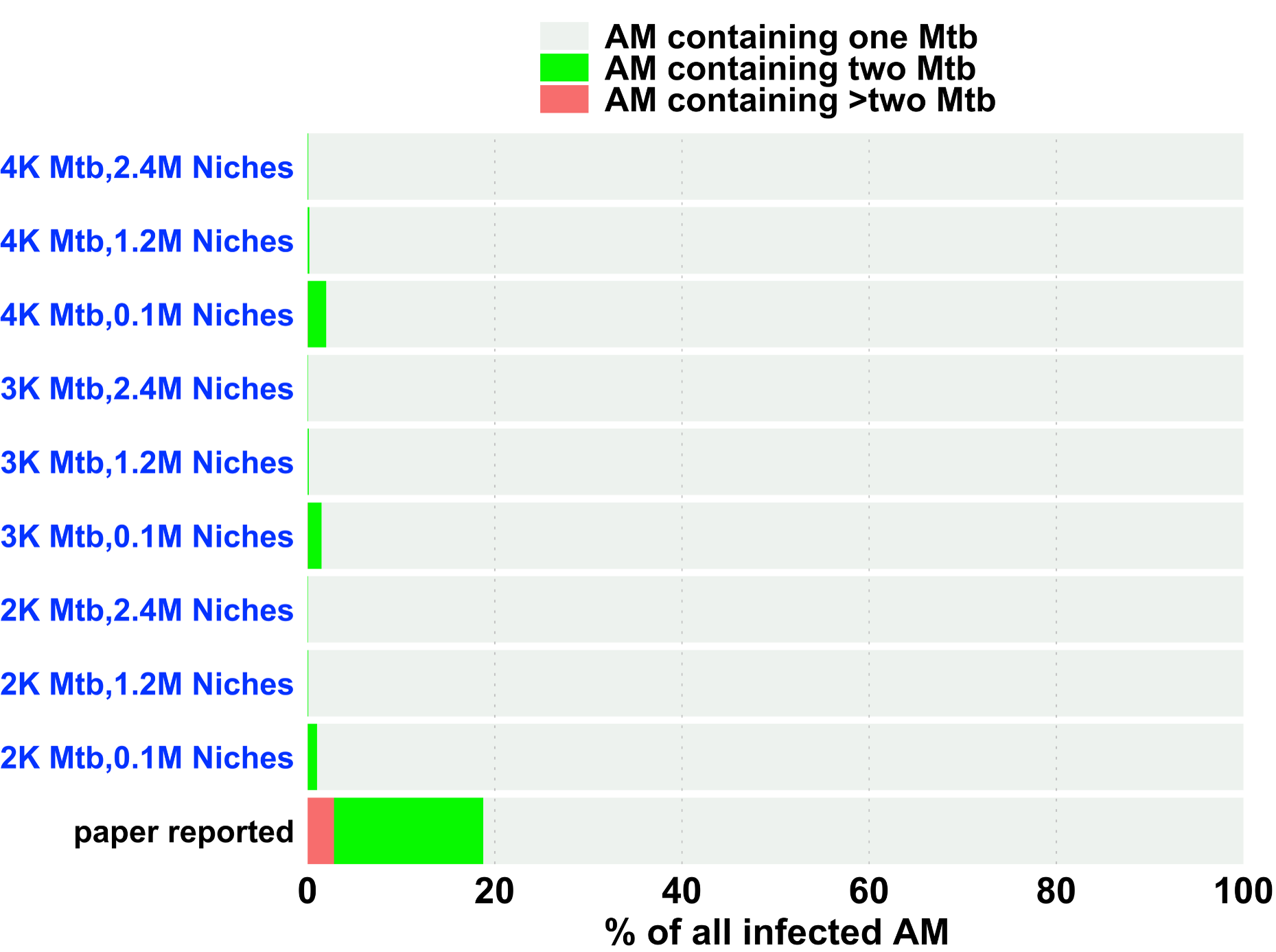
As a result, in all one million simulations, at least 85% of the niches contain a single M.tb. And the means of simulation under representitive scenarios are depicted below. Contrary to the paper reported, random depostion can only result in less than 5% niches with two M.tb but larger than 95% niches with one M.tb
Preferred deposition
Seek a function $f$ describing the probability that a pathogen will be deposited into each niche, such that the likelihood of the observation reported by the paper will be maximized, i.e. $$ \underset{f(x)}{\text{arg max}} \, L(f(x) \mid d_0) $$ where $x$ is the whole set of niches pathogens can be deposited into; $f(x)$ is the probability density function of $x$ , i.e. $f(x_i)$ is the probability that a pathogen will be deposited into the niche $x_i$ ; $d_0$ is the distribution of pathogens in the niches reported by the paper; $L(f(x) \mid d_0)$ is the likelihood of $f(x)$ given $d_0$ .
Approximate $d_0$ by $d'$ from $\underset{d' \in \mathbb{R}^2}{\arg\min} \| d' - {d_o} \|, \quad {d_o} \in \mathbb{R}^5 $ . Before enough data is available to enable a rigorous theoretical derivation, it is assumed that each droplet deposit in alveolar niches independently and $$ \begin{equation} f(x_i) = \begin{cases} P_1, & \forall i \in [1, N_{P1}] \\ P_2, & \forall i \in (N_{P1}, N_{\text{niche}}] \end{cases} \end{equation} $$ where niches were categorized into two classes and $P_i$ is the probability of being deposited of the niches belonging to i-th category. Please note adding one class will increase the computation complexity by a factor of 𝑂(𝑛) due to the added dimension. $N_{Pi}$ is the number of niches belonging to i-th category. $N_{\text{niche}}$ is the total number of niches.
A matrix $N$ below represents k-th possible scenarios that comply with $d_{0}$ , equation $(1)$ and the total number of M. tuberculosis (M.tb) deposited in the alveoli, given by $n_{Mtb} \in [2, 4] \times 10^3$ .
$$ N_k = \begin{bmatrix} N_{11} & N_{12} \\ N_{21} & N_{22} \\ \end{bmatrix} $$ Where $N_{ij}$ represents the number of niches that were deposited by $i$ (an integer) M.tb, and each M.tb is deposited with a probability of $P_j$ . Thus, the probability of $N_k$ given $N_k, d_{0}, P_1, P_2, N_{P1}, N_{\text{niche}},n_{\text{Mtb}}$ is
$$ \begin{gather*} p(N_k \mid d_{0}, P_1, P_2, N_{P1}, N_{\text{niche}}, n_{\text{Mtb}}) = P_1^{N_{11}+2N_{21}} \times P_2^{N_{12}+2N_{22}} \\ \binom{N_{\text{niche}}}{N_{P1}} \binom{N_{P1}}{N_{11}} \binom{N_{P1}-N_{11}}{N_{21}} \binom{N_{P2}}{N_{12}} \binom{N_{P2}-N_{12}}{N_{22}} \times \\ \binom{n_{\text{Mtb}}}{N_{11}+N_{12}} \times \prod_{j=0}^{\frac{n_{\text{Mtb}}^{N_2.}}{2}} \binom{n_{\text{Mtb}}^{N_2.}-2j}{2} \end{gather*} $$Where $n_{\text{Mtb}}^{N_2.}=n_{\text{Mtb}}-N_{11}-N_{12}$ is the number of M.tb deposited into niches that eventually have two M.tb at the same niche. The above formula can be reformulated to clearly reflect its dependency on the independent variables, enabling a more efficient loop design. Specifically, below parts depend on $N_k, d_{0}, P_1, P_2, N_{P1}, N_{\text{niche}},n_{\text{Mtb}}$ :
$$ \begin{equation} \binom{N_{P1}}{N_{11}} \binom{N_{P1}-N_{11}}{N_{21}} \binom{N_{P2}}{N_{12}} \binom{N_{P2}-N_{12}}{N_{22}} \end{equation} $$Below depends on $d_{0}, P_1, P_2, N_{P1}, N_{\text{niche}},n_{\text{Mtb}}$ : $$ \begin{equation} P_1^{N_{11}+2N_{21}} P_2^{N_{12}+2N_{22}} \binom{N_{\text{niche}}}{N_{P1}} \end{equation} $$
Below depends on $d_{0}, N_{\text{niche}},n_{\text{Mtb}}$ : $$ \begin{equation} \binom{n_{\text{Mtb}}}{N_{11}+N_{12}} \times \prod_{j=0}^{\frac{n_{\text{Mtb}}^{N_2.}}{2}} \binom{n_{\text{Mtb}}^{N_2.}-2j}{2} \end{equation} $$
Equation (4) can be algebraically derived into below to simplify the calculation significantly: $$ \begin{equation} \binom{n_{\text{Mtb}}}{N_{11}+N_{12}} \times {(n_{\text{Mtb}}^{N_2.})!} \prod_{j=1}^{\frac{n_{\text{Mtb}}^{N_2.}}{2}} (2j-1) \end{equation} $$
Now the probability of $N_k$ given $N_k, d_{0}, P_1, P_2, N_{P1}, N_{\text{niche}},n_{\text{Mtb}}$ can be rewriten into: $$ \begin{equation} p(N_k \mid d_{0}, P_1, P_2, N_{P1}, N_{\text{niche}}, n_{\text{Mtb}}) = e^{\ln(2) + \ln(3) + \ln(5)} \end{equation} $$ Note the values of $(2),(3),(5)$ exceed the limits that are acceptable by R or Python, but their product $(2)(3)(5) \in (0, 1)$ . And $e^{\ln(x)}$ transformation in equation (6) makes $(2)(3)(5)$ computable.
Last, the probability of $P_1, P_2, N_{P1}, N_{\text{niche}}$ given $d_{0},n_{\text{Mtb}}$ can be caculated as: $$ \begin{equation} L(f(x) \mid d_{0},n_{\text{Mtb}}) \approx L(f(x) \mid d',n_{\text{Mtb}}) = \sum_{N_k}^{} e^{\ln(2) + \ln(3) + \ln(5)} \end{equation} $$
Below are R codes to compute equation (7). First, the combinations and permutations are approximated using the Gamma function, developed by the Indian mathematician Srinivasa Ramanujan (1887–1920), which otherwise exceed the default capabilities of R and Python functions.
#necessary functions
ramanujan <- function(n){
  n*log(n) - n + log(n*(1 + 4*n*(1+2*n)))/6 + log(pi)/2
}

logCmbn<- function(n,k){
  ramanujan(n) - ramanujan(k) - ramanujan(n-k)
}

logPermute<- function(n,k){
  ramanujan(n) - ramanujan(n-k)
}
Below pre-computation to speed up:
# N is a matrix whose element Nij is the number of niches with Pj (the
# probability that a pathogen will be deposit into the niche) and occupied
# by i (an integer number, any of 1:1:3) pathogens
# N=[N11 N12
#   N21 N22
#   N31 N32]
# for N used in downstream, dim(N) is c(2,2)
# N=[N11 N12
#   N21 N22]
# CFU should be able to be calculated from N, but for speed we directly input CFU

#** k=the portion of mtb that goes to a niche of one, two or three-mtb occupied niche**
#** as reported in Fig1D **
# k<-round(c(1:3)*c(81.25,15.625,3.125)/c(c(1:3)%*%c(81.25,15.625,3.125)),3)
# k<-round(c(1:2)*c(83,17)/c(c(1:2)%*%c(83,17)),3)

pre_computed<-function(k=round(c(1:2)*c(83,17)/c(c(1:2)%*%c(83,17)),3),
               CFU=3e3L){
  #** k*CFU is the number of mtb that  goes to a niche of one, two or three-mtb occupied niche**
  #** SUMni is the number of niches that are occupied by one, two or three-mtb **
  SUMni<-as.integer(round(1/(1:length(k*CFU))*k*CFU))

  #** below pre-compute matrices or vectors to select N matrices that obeys P matrix **
  #** Ln1 is argument of f1(). **
  #** Ln1 is a 4 X I matrix, I is the number of all possible N constrained by CFU and paper's Fig1D **
  #**     Rows 1 to 4 of Ln1 is possible values of {N11}, {N12}, {N21}, {N22} respectively **
  #**

  Ln0<-reshape2::melt(matrix(nrow = SUMni[2]+1, ncol =  SUMni[1]+1))[,c("Var2","Var1")]-1L
  Ln1<-cbind(Ln0[,1],SUMni[1]-Ln0[,1],Ln0[,2],SUMni[2]-Ln0[,2])
  Ln1<-t(Ln1)#0.13s/run

  #** LsA is argument of f1(). **
  #** LsA= Ln1[1,] + Ln1[3,], i.e. N11+N21 the total number of niches that have p1 chance to be occupied**
  LsA<-Ln1[1,] + Ln1[3,]

  #** LsD is argument of f1(). **
  #** LsD= Ln1[2,] + Ln1[4,], i.e. N12+N22 the total number of niches that have p2 chance to be occupied**
  LsD<- sum(SUMni)-LsA
  # identical(Ln1[2,] + Ln1[4,],LsD)

  #logCirCle3 component,Sumini1, and Sumini2=CFU-Sumini1
  Sumini1full<-LsA+(0L:SUMni[2])

  #logCircle2 is independent of N P, and is the same for different N P as long as CFU remains the same
  logCircle2<- logCmbn(CFU,SUMni[1])+
    sum(log(seq.int(CFU-SUMni[1]-1L,1L,by = -2L)))+logPermute(SUMni[2],SUMni[2]-1)

  list(Ln1,LsA,LsD,Sumini1full,logCircle2)
}
Once we defined $f(x)$ (the matrix P in below R codes), equation (7) is calculated by:
#given CFU,seek a matrix P (which describes f(x) in the text) to maximize f1(P) which calculates equation (7) in the text
# P =[nP1,np2
#     P1 ,p2]
# rowsum(P)=[nAlveoli;]
# P[1,] %*% P[2,]=1
f1<- function(Prow1,logProw2,CFU,LsA,LsD,Ln1,Sumini1full,logCircle2){
  # f1 gets the probability given a fixed P;

  # 1. generate all possible N compatible with P and nAlveoli/pathogen distribution
  # in the paper
  l<- (LsA<=Prow1[1]) & (LsD<=Prow1[2])
  Ln<-Ln1[,l]
  Sumini1<-Sumini1full[l]

  # 2. get logCircle3 of each N
  logCircle3<-logProw2[1]*Sumini1+logProw2[2]*(CFU-Sumini1)+logCmbn(sum(Prow1),Prow1[1])

  # 3. logCircle1 of each N
  logCircle1<-getlogCircle1(Ln,Prow1)

  sum(exp(logCircle2+logCircle3+logCircle1))
}
And the getlogCircle1() is written to be more efficient than data.table using 16 threads:
getlogCircle1<-function(Ln,Prow1){
  lLn<-length(Ln)
  Ln2sbstr<-Ln
  Ln2sbstr[3:4,]<-0L
  Ln2sbstr<-c(0L,0L,Ln2sbstr[-((lLn-1):lLn)])
  #all components of logCircle1
  alllogCircle1components<-logCmbn(Prow1-Ln2sbstr,Ln)
  #get logCircle1 of each N
  #speed on mac: aggregation<data.table<built matrix+colsums
  colSums(matrix(alllogCircle1components,nrow=4),na.rm = T)
}
Stochastic gradient descent is used to seek the $f(x)$ with max likelihood, traversing the total number of M. tuberculosis (M.tb) deposited in the alveoli $n_{Mtb} \in [2, 4] \times 10^3$ :
getdP<- function(relP,P11,nNiches) {

  Prow1<- c(P11,nNiches-P11)
  crP<-f1(Prow1,log(c(1,relP)/c(c(1,relP)%*%Prow1)),CFU,LsA,LsD,Ln1,Sumini1full,logCircle2)

  Prow1d<- c(P11+100L,nNiches-P11-100L)
  dP11<-f1(Prow1d,log(c(1,relP)/c(c(1,relP)%*%Prow1d)),CFU,LsA,LsD,Ln1,Sumini1full,logCircle2)/crP-1

  relPd<-relP+0.1
  drelP<-f1(Prow1,log(c(1,relPd)/c(c(1,relPd)%*%Prow1)),CFU,LsA,LsD,Ln1,Sumini1full,logCircle2)/crP-1

  list(P11=dP11,relP=drelP,crP=crP)
}
GD<-function(relP=10,P11=2e5L,nNiches=1e6L,nItr=1e3,mrelP=0.5,mP11=0.5,
             k=round(c(1:2)*c(83,17)/c(c(1:2)%*%c(83,17)),3),
             CFU=3e3L){
  #1>mP11>0 the percentage of last dP11 contribute to new dP11
  #1>mrelP>0 the percentage of last drelP contribute to new drelP

  precomputed<-pre_computed(k,CFU)
  precomputed_names<-c('Ln1','LsA','LsD','Sumini1full','logCircle2')
  for (i in (1:length(precomputed))){
    assign(precomputed_names[i],precomputed[i])
  }

  m<-matrix(ncol = 5, nrow= nItr)
  colnames(m)<-c("relP","P11","P", "drelP","dP11")
  dP<-getdP(relP,P11,nNiches)
  if (is.na(dP$P11)) {stop("current P is 0, try set a better initializaiton")}
  if (abs(P11*dP$P11)<=1000 && abs(P11*dP$P11)>=100){
    dP11<-P11*dP$P11}
  else if (abs(P11*dP$P11)>1000) {dP11<-sign(dP$P11)*1000L}
  else {dP11<-sign(dP$P11)*100L}

  if (abs(relP*dP$relP)<=1 && abs(relP*dP$relP)>=0.1){
    drelP<-relP*dP$relP}
  else if (abs(relP*dP$relP)>1) {drelP<-  sign(dP$relP)}
  else {drelP<-  sign(dP$relP)*0.1}

  m[1,]<-c(relP,P11,dP$crP,drelP,dP11)
  relP<-relP+drelP
  P11<-round(P11+dP11)

  for (i in 2:nItr) {
    tm<-proc.time()
    dP<-getdP(relP,P11,nNiches)
    if (abs(P11*dP$P11)<=1000 && abs(P11*dP$P11)>=100){
      dP11<-mP11*dP11+(1-mP11)*P11*dP$P11}
    else if (abs(P11*dP$P11)>1000) {dP11<-mP11*dP11+(1-mP11)*sign(dP$P11)*1000L}
    else {dP11<-mP11*dP11+(1-mP11)*sign(dP$P11)*100L}

    if (abs(relP*dP$relP)<=1 && abs(relP*dP$relP)>=0.1){
      drelP<-mrelP*drelP+(1-mrelP)*relP*dP$relP}
    else if (abs(relP*dP$relP)>1) {drelP<-mrelP*drelP+(1-mrelP)*sign(dP$relP)}
    else {drelP<- mrelP*drelP+(1-mrelP)*sign(dP$relP)*0.1}

    m[i,]<-c(relP,P11,dP$crP,drelP,dP11)

    relP<-relP+drelP
    P11<-round(P11+dP11)
    cat("iteration",i,"done",(proc.time()-tm)[3],"s\n")
  }
  return(m)
}
Result
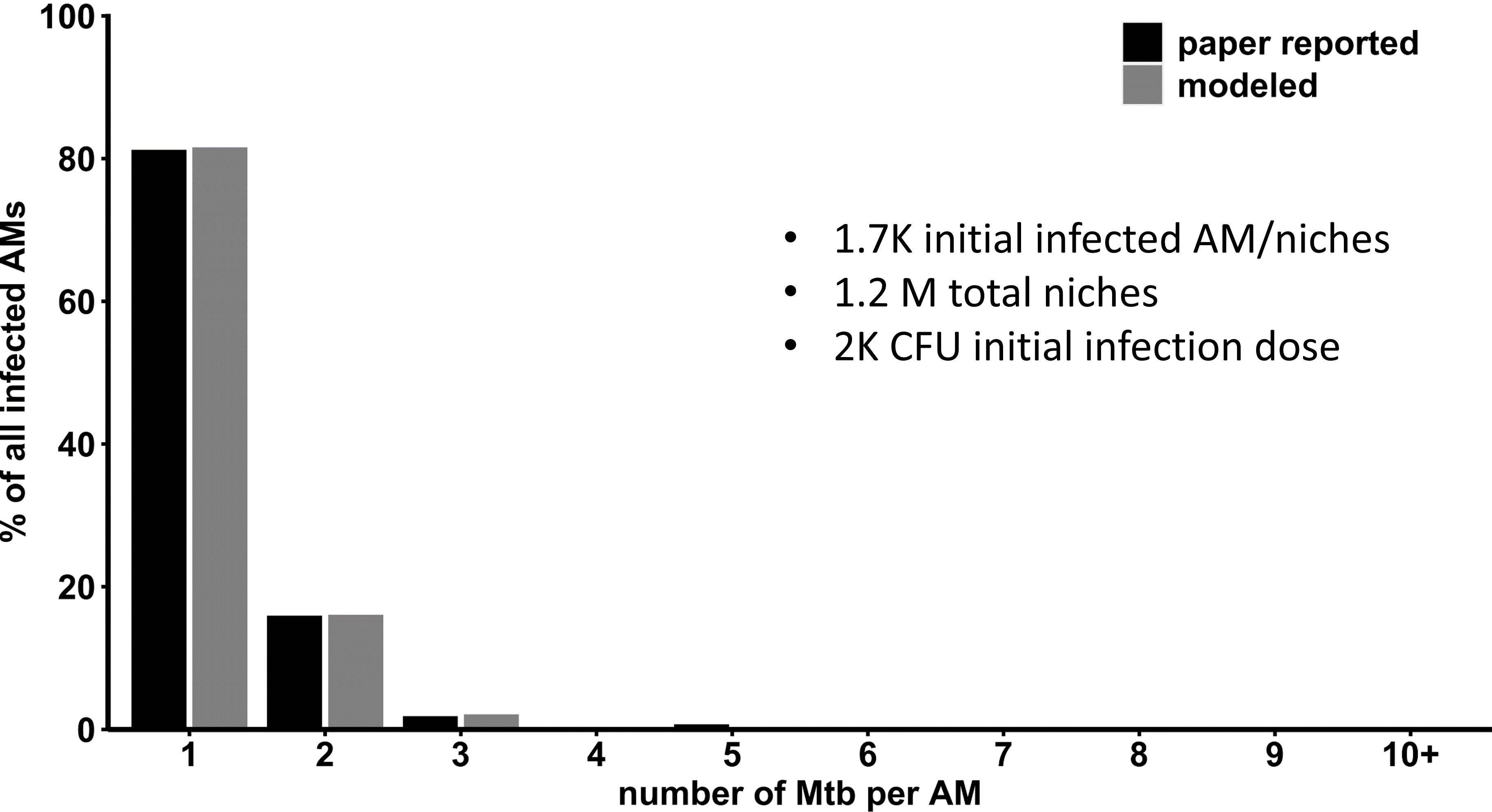
As a result, Monte Carlo simulation using the $f(x)$ of max likelihood gives a nealy same result as reported in the Fig 1D of Rothchild et al.,(2019).

Animated visulization
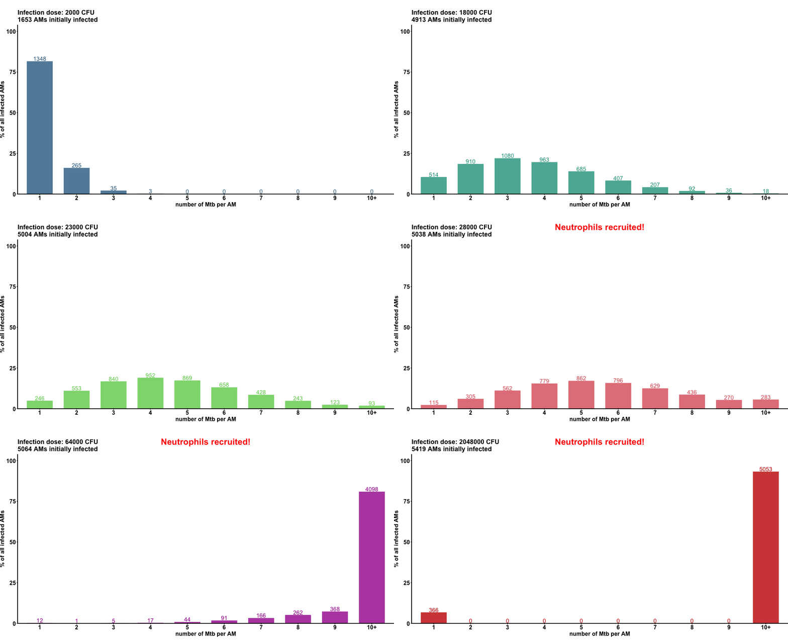
We can continue to predict the the number of alveolar macrophages initially infected varied with infection dose, and what infection dose can cause acute symptomatic infection. Below animation demonstrates the prediction.